8. Variation With Speaker
Learning Objectives
- to appreciate the range of acoustic properties of speech that vary across speakers (for the same linguistic message)
- to understand some of the challenges in making robust and reliable speaker identification on the basis of acoustic measurements
- to understand how speaker identification is performed within a forensic framework, including Bayesian methods
- to understand how automatic speaker identification is performed, including Gaussian Mixture Models
- to gain experience with the construction of a speaker recognition system
- to gain experience in attempting to disguise a voice
Topics
- Why study speaker variety?
Different speakers produce the same utterance with the same meaning in different ways. This highlights two important characteristics of speech communication: that speakers' performances vary and that listeners are able to cope with that variability. Speakers not only differ in terms of vocal tract and larynx size, but at all linguistic levels, and that understanding that variability might help us understand how linguistic levels are organised. Listeners are known to adapt to speakers and to accents - a better understanding of these processes may be useful in building better-performing speech technology. Speaker identity can be important in criminal cases, where two speech recordings may need to be judged in terms of whether they could have been produced by the same speaker. Applications that exploit speaker identity, such as Forensic Phonetics or Biometrics need better quantitative models of the expression of identity in voice.
- Speaker Variation
Variations across speakers
Speakers vary, of course, at a physiological/anatomical level, with differences in the sizes of their vocal tract and larynx, and this can affect fundamental frequency range, voice qualities, formant frequencies and spectral shaping generally. But they also vary in that each has learned habits about preferred ways of speaking, which might include default gestural settings and idiosyncratic articulatory gestures. Overall gestural “settings” (like jaw position, lip spreading, nasality, etc) can affect global aspects of the speech, while speakers can also be idiosyncratic with regard to their realisation of particular phonological elements at segmental or supra-segmental levels (see Nolan 2009 for discussion). Speakers may also vary in the precise details of the phonological system they inferred as learners from their L1, not just in terms of accent, but in terms of the pronunciation specification of lexical forms. Second language speakers are strongly influenced by language habits learned for their first language. For speaker identification by voice, the hope is that these idiosyncrasies are sufficient to distinguish the speaker from others.
Typical acoustic properties
In trying to characterise the sounds made by a speaker, a lot of weight is usually put on spectral envelope features, since these reflect both the vocal tract size and the gestural habits of the speaker for different phonological segments. However global properties such as speaking rate, dysfluency rate, mean fundamental frequency and fundamental frequency distribution are also widely used. Other voice quality features are used less, perhaps because they are hard to extract reliably from the acoustic signal.
Challenges to speaker identification
A number of problems arise from variation in the acoustic environment in which the speech is recorded. It can be difficult to know whether differences in recordings are due to changes of speaker or changes of channel. This is true for both human and machine identification. Also some acoustic parameters are strongly affected by noise, for example, voice quality measures such as jitter and HNR are very sensitive to audio quality. But the biggest problem comes from the fact that speech is a performance and that speakers have a lot of freedom to change the way they speak in a given situation. Speech sounds may be influenced by unique characteristics of the speaker, but no single aspect of the signal invariantly identifies the speaker.
- Application: Forensic Phonetics
Forensic voice comparison
Voice experts can be called upon to compare two or more speech recordings collected in criminal cases, for example a recording of the criminal and a recording of a suspect. The expert is asked his opinion as to whether it is possible (or likely) that the two recordings could have been made by the same speaker (see Nolan 2001 for legal discussion). Experts will use their own auditory phonetic judgements by listening for idiosyncratic characteristics like voice quality, speaking style and accent, often backed up by instrumental measurements of formant frequencies and prosody.
Forensic Phonetics has a chequered history because of the claim made by some authorities that "Voiceprints" (i.e. spectrograms) are as accurate as fingerprints for identification. This is clearly untrue, since fingerprints are part of your body while speaking is a performance. Just because you can choose between a few of your friends and relations from their voice does not mean that all speakers have unique voices, nor that speakers are recognisable in all circumstances. Forensic Phoneticians sometimes have to stand up in court and justify the procedures they have used and the conclusions they have drawn, it is beholden on them to be honest about the reliability and efficacy of their techniques. Unfortunately such high professional standards have not always been attained. Forensic Phonetics is currently under pressure to become more "scientific", with better use of statistical measures and Bayesian methods of likelihood estimation (see Rose, 2003).
Forensic voice line-ups
Determining the identity of speakers from their voice is found in another forensic area. This is where the voice of the criminal was not recorded at the scene of the crime, but was heard by a witness to the crime (an ear-witness). If the police have a suspect for the crime, they might present a recording of the suspect to the witness. To try to avoid bias, this is usually done in the form of a voice line-up.
A voice line-up is like an identity parade; the voice of the suspect is included in a list of distractor voices collected from non-suspects. The witness to the crime listens to all the voices in random order then picks out the voice they remember from the line-up.
While apparently scientific, the voice line-up is not without problems. For example, how are the distractor voices chosen? What if the suspect has a distinctive accent or voice quality - should the distractors be chosen to have the same? Many experiments have shown that listeners have a very poor memory for the qualities of speaker voices, and the results of a voice line up need to be interpreted with care. A famous criminal case involving voice identification was the Lindbergh baby kidnapping case.
- Application: Speaker recognition systems
Speaker Recognition
Automatic systems for recognising speakers are of two types:
- speaker identification systems select one speaker from N known speakers on the basis of their voice;
- speaker verification systems confirm the identity of a single named speaker on the basis of their voice.
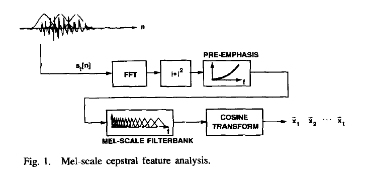
Speaker verification systems are more widely employed at the present time, to authenticate access to buildings or bank accounts for example. The technology for speaker verification is well developed and is quite robust (see Reynolds, 1995) with error rates around 1% in laboratory tests (i.e. 1% false rejects and 1% false acceptances). Systems can be divided into text-dependent and text-independent systems, the former being of better performance. In a typical system, speakers enrol by recording some known sentences - say a few minutes of speech in total. From the enrolment recordings a statistical model is made of the spectral envelopes used by each speaker. In addition a population model is built from the combination of all enrolled speakers. In identification, a challenge recording is compared to each statistical model and the best fitting model chosen. In verification, the probability that the supposed speaker's model produced the speech is compared with the probability that the population model produced the speech. Only if the speech is more likely to have been produced by this speaker than by anyone in the population would the speaker's identity be confirmed. A Gaussian Mixture Model (GMM) is the most commonly used form of statistical model in speaker recognition. Cepstral coefficients are the most common form of spectral envelope parameters.
System Design
Robust text-independent speaker recognition is possible through the use of MFCC features to describe the spectral envelope, GMMs to model the acoustic probability space, and Bayes' theorem for inference:
Acoustic feature analysis:
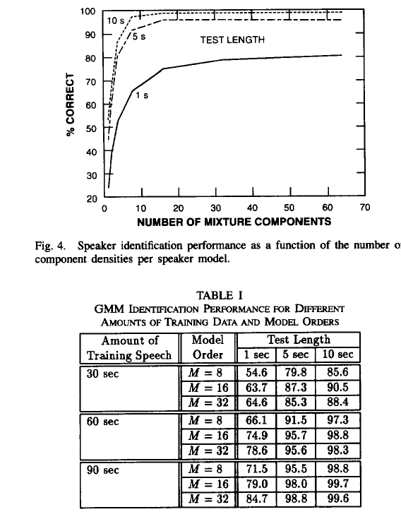
Performance on a 16-speaker database using mel-scaled cepstral coefficients (D. Reynolds & R. Rose, 1995):
- Application: Voice disguise
Systems for disguising the voice are sometimes useful in legal cases where the identity of a witness needs to be hidden. Typically disguise uses pitch shifting and spectral warping tools developed for the music industry. These can change the apparent larynx size and vocal tract size of the speaker, and hide some aspects of voice quality. However they are not very effective at disguising accent. Testing the effectiveness of voice disguise and evaluating the performance of human listeners for speaker identification are active areas of research.
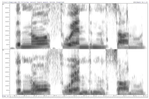
Disguise of female voice (top) by vocal tract length scaling and pitch scaling (bottom).
- Technique: Gaussian Mixture Models
A Gaussian probability density function is the proper name for the normal distribution - the bell-shaped curve that is ubiquitous in studies of the distribution of naturally-occurring measurements. In the one dimensional case, the Gaussian pdf is described by two parameters: the mean μ and the variance σ2. However if the distribution is not bell-shaped, then one Gaussian does not provide a good description, and so we use multiple Gaussian curves to model the data:
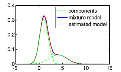
The overall distribution is then modelled by a mixture of Gaussians, each mixture component is a single Gaussian curve, and the relative importance of each mixture is recorded in the prior probabilities of each mixture, called the mixture weights.
In the multi-dimensional case, each measurement is now a vector of data values (energies in different frequency bands, for example), and the concept of a Gaussian distribution is extended to deal with a cloud of points having a centre and a variability along each direction in the vector space. Here is an example of a 3-mixture model in two dimensions:
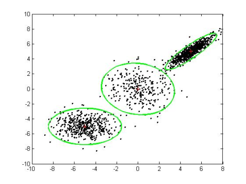
There exist robust, iterative algorithms for finding the best fitting means, variances and mixture weights for modelling a set of multi-dimensional data vectors. From the model we can then calculate the probability that a new vector was part of the distribution used to train the model.
- Technique: Bayes' Theorem
Bayes' theorem is an application of the laws of conditional probability. Say we have two classes of event: A and B; there are situations where A arises by itself, B arises by itself, A & B arise together, and when neither A or B arise:
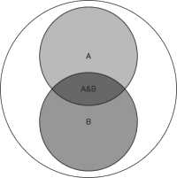
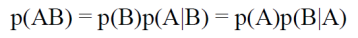
We write the probability of A occurring as p(A), and the probability of B occurring as p(B). We write the probability of A and B occurring together as p(AB). Now we can calculate p(AB) in two ways, either by taking p(B) and asking how often A is present given that B has occurred, or by taking p(A) and asking how often B is present given that A has occurred. That is
Read p(A|B) as the probability of A given that B has occurred. Bayes' theorem is just a rearrangement of this into the wonderful:
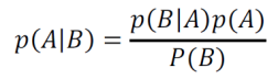
Which allows us to calculate a posterior probability p(A|B) from the likelihood p(B|A) in combination with the priors p(A) and p(B).
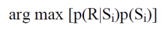
Say we have a recording R, and we want to know the probability that it was produced by speaker S, that is p(S|R). Bayes' theorem says that we can calculate this if we know
- p(R|S) that is the probability that this recording could have been produced by S (this is the role played by the Gaussian Mixture Model)
- p(S) that is the prior probability that S could be the speaker
- p(R) that is the prior probability that this recording could have occurred
If we only want to compare the probability of different speakers {Si} for the same R, then p(R) is a constant, so we can find the most likely speaker from:
In speaker verification we compare the probability that R could have been produced by the proposed speaker S, that is p(S|R), with the probability that R could have been produced by anyone from a population G of speakers, p(G|R). This ratio of probabilities is just
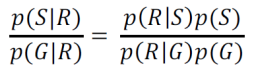
If this ratio is greater than some threshold, then the speaker is accepted. The part of the expression p(R|S)/p(R|G) is called the likelihood ratio.
References
- F. Nolan, The Phonetic Bases of Speaker Recognition, Cambridge University Press, 2009.
- D. Reynolds & R. Rose, "Robust text-independent speaker recognition using gaussian mixture speaker models", IEEE Trans. Speech and Audio Processing 3 (1995), 72-83. On Moodle.
- R. Rose, The technical comparison of forensic voice samples, in Expert Evidence, 2003. On Moodle.
Readings
- V. Dellwo, M. Ashby, M. Huckvale, "How is individuality expressed in voice? An introduction to speech production & description for speaker classification", in Speaker Classification I, C.Mueller (ed), Springer Lecture Notes in Artificial Intelligence, 2007. On Moodle.
- F. Nolan, "Speaker identification evidence: its forms, limitations, and roles", Proceedings of the conference 'Law and Language: Prospect and Retrospect', December 12-15 2001, Levi (Finnish Lapland). On Moodle.
- Anders Eriksson, “Tutorial on Forensic Speech Science”. On Moodle.
Laboratory Exercises
- Take part in a voice line-up
- A number of voices will be played to you to see if you can identify a speaker.
- Testing a speaker recognition system
- Check your microphone is switched on and working.
- Run the "recspeaker" application found in y:/EP/recspeaker and check that the "library" folder is set to "y:\recog":
- Select the "Recognise Me" button. You will be prompted to make a short recording. Click the "Record" button to start recording, which will stop automatically after 10s.
- When you click the "Done" button, your recording will be processed into cepstral coefficients and compared with a set of GMM models in the library folder. The recognition results are then displayed. You will see scores that compare your voice to the stored models. Larger scores mean a better match.
- The stored models were generated from your recordings of the BKB sentences we made in week 1. You can enrol your voice again using the "Enrol Me" opion of recspeaker. On the opening screen click the "Enrol Me" button. On the next screen, enter your name and click "Record" to make a recording of the given text. The recording will stop automatically after 30s. When you click "Done", a GMM will be built from your recording and added to the library. You can now ask the system to recognise you again. You will probably find that you are better recognised (i.e. a higher score) than before. Why do you think that is?
- Try recording a different text than the one suggested. Does the system still recognise you?
- Try "putting on a different voice". Does the system still recognise you?
- What might make systems like this unreliable?

- Investigating an impersonation
- In y:/EP/ you will find two recordings, one of a genuine speaker (connery-real.sfs) and one of an impersonation (connery-impersonation.sfs).
- How good is the impersonation?
- What characteristics of the original voice form the basis for the impersonation?
- What doesn't work well in the impersonation?
- Investigating Voice Disguise
- Using WASP, record a sample of your speech at 22050 samples/sec. Save the audio to a WAV file on the desktop.
- Run the program y:/EP/VoiceTest.exe and use File|Open to open your recording. Select Audio|Play to play your recording. Move the sliders to disguise your voice.
- The sliders work as follows: Size changes the effective vocal tract length of the speaker by scaling the spectral frequencies (independently of pitch); Pitch scales the pitch of the voice; Tilt changes the spectral slope; Rough increases the amount of creakiness in the voice (left) or increases the amount of breathiness in the voice (right).
- Try out changes to the sliders to find a combination that best disguises your identity. Explain why you think your final settings work best.
Reflections
- Think of factors that might affect the reliability of earwitness evidence.
- What criteria should one use to choose "foils" for a voice line-up?
- Why might the performance of a speaker recognition system in the laboratory not be a good predictor for its performance in the field?
- Why are spectral-envelope measures used in automatic speaker recognition rather than formant frequencies, fundamental frequency or voice quality measures?
Word count: . Last modified: 12:23 01-Mar-2018.